Sentiment analysis in Spanish
Note: (This is a continuation of a previous article in which I explained how to download and plot a heatmap of thousand of tweets sent from my hometown.)
You can find the code I used for this tutorial in github. I also uploaded the tweets file so you can follow along without having to download the tweets by yourself.
On this post, I will focus on how to perform Sentiment Analysis on a Spanish corpus.
In terms of SA, currently is very easy to apply it on English corpus. The TextBlob package comes with a pretrained model, as well as word2vec.
However, as far as I can tell, there are no pretrained models in Spanish.
So I decided to build the model by myself.
In order to do so, I needed a labeled dataset. I used the TASS DATASET.
TASS is a Sentiment Analysis in Spanish Workshop hosted by the Spanish Society for Natural Language Processing (SEPLN) every year. To use it you have to request permission (send an email to ), hence I can't share the corpus here. Reach out to them if you are interested, I'm sure they will help you out.
They have multiple XML files containing thousands of tweets in spanish with their associated polarity. Some of the files are focused on a specific topic, such as Politics or TV.
The structure of one of the files looks like:
<?xml version="1.0" encoding="UTF-8"?>
<tweets>
 <tweet>
  <tweetid>142378325086715906</tweetid>
  <user>jesusmarana</user>
  <content><![CDATA[Portada 'Público', viernes. Fabra al banquillo por 'orden' del Supremo; Wikileaks 'retrata' a 160 empresas espías. http://t.co/YtpRU0fd]]></content>
  <date>2011-12-02T00:03:32</date>
  <lang>es</lang>
  <sentiments>
   <polarity><value>N</value></polarity>
  </sentiments>
  <topics>
   <topic>política</topic>
  </topics>
 </tweet>
 <tweet>
So we are mostly interested on the content field and the sentiment.polarity.value.
Be aware that the schema varies depending on which year's dataset you are reading.
After parsing and joining all available datasets, that left me with a dataset containing over 48,000 tweets with an associated sentiment. Sentiment is encoded as an ordinal variable containing one of the following: N+ (very negative), N (negative), NEU (Neutral), P (Positive), P+ (very positive).
The goal is to predict the polarity of the tweet file we processed on the previous blog post by using our labeled dataset.
However, before doing that, there is another step we have to take.
If we start browsing downloaded tweets, we will notice that something is wrong. We cannot use the TASS corpus to predict sentiment on tweets that are not in spanish.
Which means we have to perform language detection on the tweets.
Language detection
To do so, I used 2 different libraries langdetect and langid, and kept only those tweets which both libraries classified as being written in Spanish.
import langid
from langdetect import detect
import textblob

def langid_safe(tweet):
    try:
        return langid.classify(tweet)[0]
    except Exception as e:
        pass

def langdetect_safe(tweet):
    try:
        return detect(tweet)
    except Exception as e:
        pass

def textblob_safe(tweet):
    try:
        return textblob.TextBlob(tweet).detect_language()
    except Exception as e:
        pass

#This will take a looong time
tweets['lang_langid'] = tweets.tweet.apply(langid_safe)
tweets['lang_langdetect'] = tweets.tweet.apply(langdetect_safe)
tweets['lang_textblob'] = tweets.tweet.apply(textblob_safe)

tweets.to_csv('tweets_parsed2.csv', encoding='utf-8')

tweets = tweets.query("lang_langdetect == 'es' or lang_langid == 'es' or lang_langtextblob=='es' ")
That left me with 48,606 tweets geocoded and written in Spanish ready to be analyzed.
Like I said above, the data set contains 'levels' of sentiment, not only positive/negative. However, since some of the files from older TASS only have Positive or Negative, I binarized the sentiment. So instead of having a 5-class classification problem we turn it into a binary one (Positive=1, Negative=0).
Text processing
To be able to manage the tweets, we need to extract information from the text. To do so, we will use scikit learn's CountVectorizer.
It will turn text into a matrix of token counts, (token being the text's words).
So for example, if we have a tweet like:
Machine Learning is very cool
CountVectorizer will turn it into:
| tweet | machine | learning | is | very | cool | |
|---|---|---|---|---|---|---|
| 0 | Machine Learning is very cool | 1 | 1 | 1 | 1 | 1 |
| 1 | Machine Learning is cool | 1 | 1 | 1 | 0 | 1 |
This way we wan work with those vectors instead of with raw text.
We will do some processing to the text as well, namely:
- Tokenize. This means applying a function that splits a text into a list of words. We will use a custom tokenizer that not only tokenizes (using
nltk.word_tokenize), but removes puntiation. In this case it is important to include¿and¡(spanish exclamation points). - Turn all words to lowercase
- Remove stopwords. Stopwords are that set of common words that have little semantical meaning. Examples of stopwords in english would be of, in, or, at ...
- Stem the words. This means that for each word, we just keep the stem) of the word. For example, beautiful, beautifully and beauty would be turn into their stem, beauti.
Here is the code to process the text.
#You have to download the spanish stopwords first with nltk.download()
import nltk
from nltk.corpus import stopwords
from nltk import word_tokenize
from nltk.data import load
from nltk.stem import SnowballStemmer
from string import punctuation
from sklearn.feature_extraction.text import CountVectorizer


#stopword list to use
spanish_stopwords = stopwords.words('spanish')

#spanish stemmer
stemmer = SnowballStemmer('spanish')

#punctuation to remove
non_words = list(punctuation)
#we add spanish punctuation
non_words.extend(['¿', '¡'])
non_words.extend(map(str,range(10)))

stemmer = SnowballStemmer('spanish')
def stem_tokens(tokens, stemmer):
    stemmed = []
    for item in tokens:
        stemmed.append(stemmer.stem(item))
    return stemmed

def tokenize(text):
    # remove punctuation
    text = ''.join([c for c in text if c not in non_words])
    # tokenize
    tokens =  word_tokenize(text)

    # stem
    try:
        stems = stem_tokens(tokens, stemmer)
    except Exception as e:
        print(e)
        print(text)
        stems = ['']
    return stems

vectorizer = CountVectorizer(
                analyzer = 'word',
                tokenizer = tokenize,
                lowercase = True,
                stop_words = spanish_stopwords)
Model Evaluation
On this step we try multiple Machine Learning Classifiers and measure their performance. Tools like SciKit-Learn Laboratory (SKLL) can help accelerate this step.
One thing we have to consider is the measure that we will use to determine wether a model is better than other. In binary classification problems a good metrics is the Area Under the Curve, which takes into account the True Positive Rate as well as the False Positive Ratean awesome measure that you should totally read about.
In my case I chose a Linear Support Vector Machine Classifier, since I have found it performs pretty well in this kind of problems.
Once we have our Vectorizer and Classifier, its a matter of fine tuning their hyperparameters to find those that perform best.
To do so, we go ahead and perform a grid search using scikit-learn GridSearchCV.
This method perform an exaustive search of the parameters specified and return a model with the best performan parameters.
This is the code that performs the search:
vectorizer = CountVectorizer(
                analyzer = 'word',
                tokenizer = tokenize,
                lowercase = True,
                stop_words = spanish_stopwords)

pipeline = Pipeline([
    ('vect', vectorizer),
    ('cls', LinearSVC()),
])


# here we define the parameter space to iterate through
parameters = {
    'vect__max_df': (0.5, 1.9),
    'vect__min_df': (10, 20,50),
    'vect__max_features': (500, 1000),
    'vect__ngram_range': ((1, 1), (1, 2)),  # unigrams or bigrams
    'cls__C': (0.2, 0.5, 0.7),
    'cls__loss': ('hinge', 'squared_hinge'),
    'cls__max_iter': (500, 1000)
}


grid_search = GridSearchCV(pipeline, parameters, n_jobs=-1 , scoring='roc_auc')
grid_search.fit(tweets_corpus.content, tweets_corpus.polarity_bin)
You can see that we can not only find parameters for the LinearSVC Classifier, but also for the Vectorizer itself.
This step will take some time. After it's done, it will return the set of parameters that return the highest AUC score. In this case, the highest AUC was 0.92. Which it is ok.
After that, we just need to train the model on the TASS corpus, load our tweets and predict the sentiment.
After that, we save the tweets latitude, longitude and polarity to a file and plot the heatmap following a similar method than what I explained on the previous post.
You could do that by using the grid_search object you used for the parameter search.
In my case, my laptop ran out of battery before I saved the model so I just recreated it by building a pipeline with the vectorizer and the LinearSVC tuned with the best params provided by the grid search.
from sklearn.svm import LinearSVC
from sklearn.pipeline import Pipeline

#we build a Pipeline object
pipeline = Pipeline([
    ('vect', CountVectorizer(
            analyzer = 'word',
            tokenizer = tokenize,
            lowercase = True,
            stop_words = spanish_stopwords,
            min_df = 50,
            max_df = 1.9,
            ngram_range=(1, 1),
            max_features=1000
            )),
    ('cls', LinearSVC(C=.2, loss='squared_hinge',max_iter=1000,multi_class='ovr',
             random_state=None,
             penalty='l2',
             tol=0.0001
             )),
])

#we fit the pipeline with the TASS corpus
pipeline.fit(tweets_corpus.content, tweets_corpus.polarity_bin)
#now we predict on the new tweets dataset
tweets['polarity'] = pipeline.predict(tweets.tweet)
Once we have the tweets with their polarity, we follow similar steps than we did on the previous twitter heatmap tutorial and we get the following heatmap of positive and negative places in Murcia (the image is pretty big, you might want to zoom in):
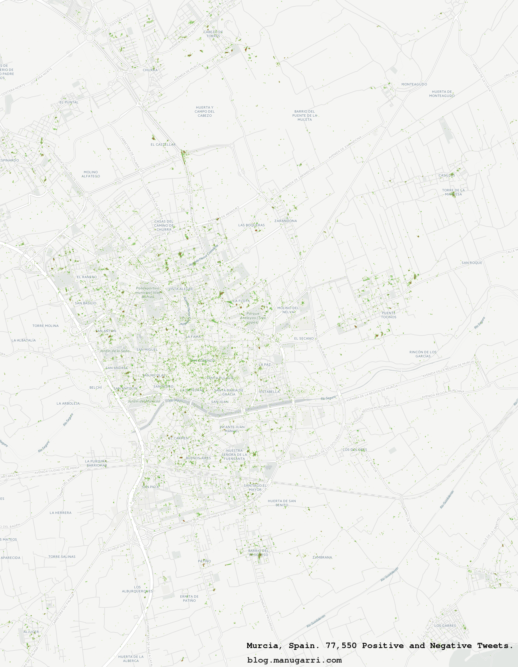
Neat, isn't it?